Fit a brokenstick model to irregular data — brokenstick • brokenstick

The brokenstick() function fits an irregularly observed series of measurements onto a user-specified grid of points (knots). The model codes the grid by a series of linear B-splines. Each modelled trajectory consists of straight lines that join at the chosen knots and look like a broken stick. Differences between observations are expressed by a random effect per knot.

Usage

brokenstick(
  formula,
  data,
  knots = NULL,
  boundary = NULL,
  k = 5L,
  degree = 1L,
  method = c("kr", "lmer"),
  control = set_control(method = method, ...),
  na.action = na.exclude,
  light = FALSE,
  hide = c("right", "left", "boundary", "internal", "none"),
  ...
)

Arguments

formula: A formula specifying the outcome, the predictor and the group variable in data. The generic shape is formula = y ~ x | group. The left-hand side is the outcome, the right-hand side the predictor, and the name of the grouping variable occurs after the | sign. Formula treatment is non-standard: 1) y and x should be numeric, 2) only one variable is allowed in each model term (additional variables will be ignored).
data: A data frame or matrix containing the outcome (numeric), predictor (numeric) and group (numeric, factor, character) variable.
knots: Optional, but recommended. Numerical vector with the locations of the internal knots to be placed on the values of the predictor. The function sorts the internal knots in increasing order.
boundary: Optional, but recommended. Numerical vector of length 2 with the left and right boundary knot. The boundary setting is passed to splines::bs() as the Boundary.knots argument. If not specified, the function determines the boundary knots as range(x). When specified, the boundary range is internally expanded to include at least range(knots).
k: Optional, a convenience parameter for the number of internal knots. If specified, then k internal knots are placed at equidense quantiles of the predictor. For example, specifying k = 1 puts a knot at the 50th quantile (median), setting k = 3 puts knots at the 25th, 50th and 75th quantiles, and so on. If the user specifies both k and knots arguments then knots takes precedence. The default is k = 5, so if the user does not specify any of knots, boundary or k, then the knots will be at the 16th, 33th, 50th, 66th and 84th quantile of the predictor.
degree: the degree of the spline. The broken stick model requires linear splines, so the default is degree = 1. Setting degree = 0 yields (crisp) dummy coding, and one column less than for degree = 1. The brokenstick package supports only degree = 0 and degree = 1.
method: Estimation method. Either "kr" (for the Kasim-Raudenbush sampler) or "lmer" (for lme4::lmer()). Version 1.1.1.9000 changed the default to method = "kr".
control: List of control options returned by set_control() used to set algorithmic details. A list with parameters. When not specified, the functions sets to defaults for method "kr" by control_kr(), and for method "lmer" by lme4::lmerControl(). For ease of use, the user may set individual options to "kr" (e.g. niter = 500) via the ... arguments.
na.action: A function that indicates what lme4::lmer() should so when the data contain NAs. Default set to na.exclude. Only used by method "lmer".
light: Should the returned object be lighter? If light = TRUE the returned object will contain only the model settings and parameter estimates and not store the data, imp and mod elements. The light object can be used to predict broken stick estimates for new data, but does not disclose the training data and is very small (often <20 Kb).
hide: Should output for knots be hidden in get, print, summary and plot functions? Can be "left", "right", "boundary", "internal" or "none". The default is "right".
...: Forwards arguments to control_kr().

Value

A object of class brokenstick.

Details

The choice between method = "kr" and method = "lmer" depends on the size of the data and the complexity of the model. In general, setting method = "lmer" can require substantial calculation time for more complex models (say > 8 internal knots) and may not converge. Method "kr" is less sensitive to model complexity and small samples, and has the added benefit that the variance-covariance matrix of the random effects can be constrained through the cormodel argument. On the other hand, "lmer" is the better-researched method, and is more efficient for simpler models and datasets with many rows.

The default algorithm since version 2.0 is the Bayesian Kasim-Raudenbush sampler (method = "kr"). The variance-covariance matrix of the broken stick estimates absorbs the relations over time. The "kr" method allows enforcing a simple structure on this variance-covariance matrix. Currently, there are three such correlation models: "none" (default), "argyle" and "cole". Specify the seed argument for reproducibility. See control_kr() for more details.

The alternative method = "lmer" fits the broken stick model by lme4::lmer(). With this method, the variance-covariance matrix can only be unstructured. This estimate may be unstable if the number of children is small relative to the number of specified knots. The default setting in lme4::lmerControl() is check.nobs.vs.nRE= "stop". The [set_control()] function changes this to check.nobs.vs.nRE= "warning" by default, since otherwise many broken stick models would not run at all. The method throws warnings that estimates are not stable. It can be time for models with many internal knots. Despite the warnings, the results often look reasonable.

Diagnostics with coda and lme4: The function returns an object of class brokenstick. For method = "kr" the list component named "mod" contains a list of mcmc objects that can be further analysed with coda::acfplot(), coda::autocorr(), coda::crosscorr(), coda::cumuplot(), coda::densplot(), coda::effectiveSize(), coda::geweke.plot(), coda::raftery.diag(), coda::traceplot() and the usual plot() and summary() functions. For method = "lmer" the list component named "mod" contains an object of class lme4::merMod. These model objects are omitted in light brokenstick objects.

Note

Note that automatic knot specification is data-dependent, and may not reproduce on other data. Likewise, knots specified via k are data-dependent and do not transfer to other data sets. Fixing the model requires specifying both knots and boundary.

Examples

# \donttest{
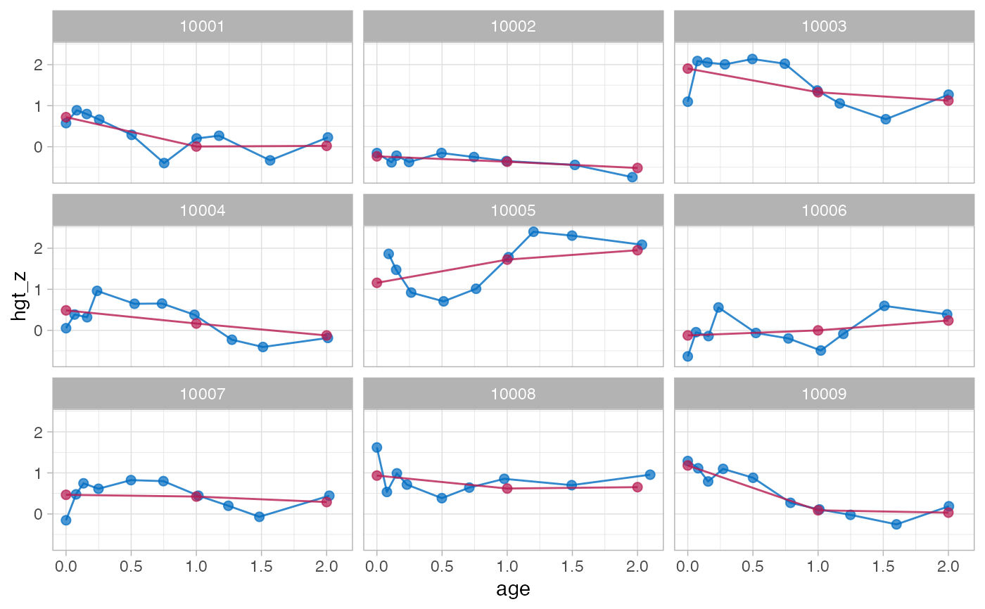
data <- smocc_200[1:1198, ]

# using kr method, default
f1 <- brokenstick(hgt_z ~ age | id, data, knots = 0:2, seed = 123)
plot(f1, data, n_plot = 9)


# study sampling behaviour of the sigma2 parameter with coda
library("coda")
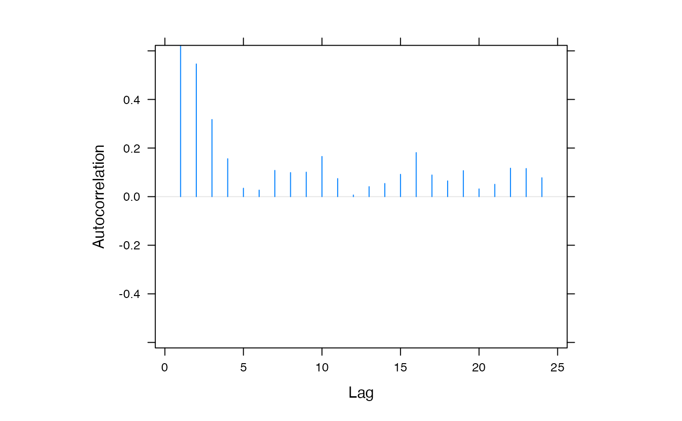
plot(f1$mod$sigma2)

acfplot(f1$mod$sigma2)


# using lmer method
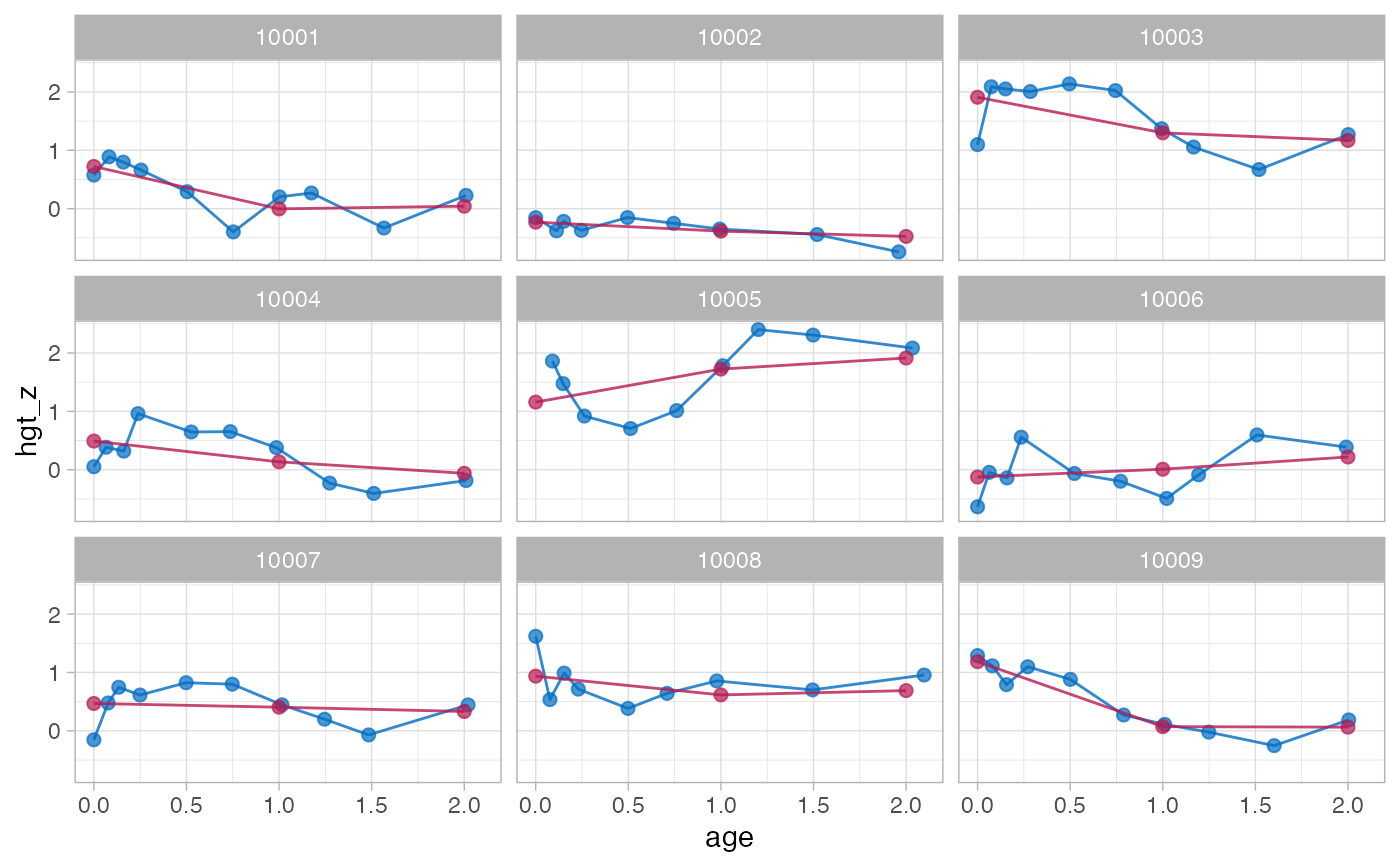
f2 <- brokenstick(hgt_z ~ age | id, data, knots = 0:2, method = "lmer")
plot(f2, data, n_plot = 9)


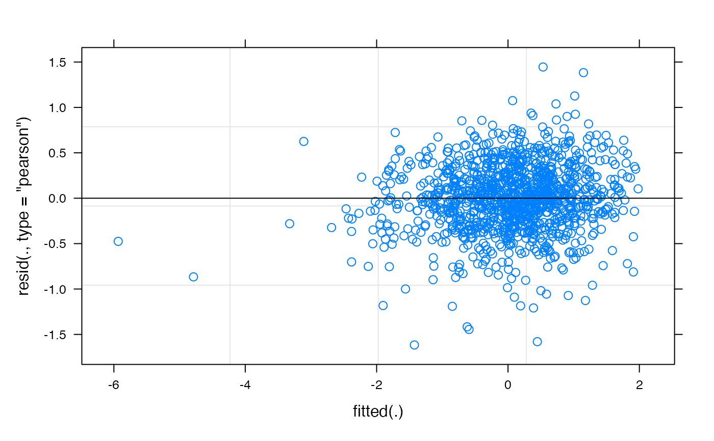
# drill down into merMod object with standard diagnostics in lme4
summary(f2$mod)
#> Linear mixed model fit by REML ['lmerMod']
#> Formula: hgt_z ~ 0 + age_0 + age_1 + age_2 + age_2.6776 + (0 + age_0 +  
#>     age_1 + age_2 + age_2.6776 | id)
#>    Data: data
#> Control: control
#> 
#> REML criterion at convergence: 2088.7
#> 
#> Scaled residuals: 
#>     Min      1Q  Median      3Q     Max 
#> -3.8278 -0.5279  0.0025  0.5652  3.4227 
#> 
#> Random effects:
#>  Groups   Name       Variance Std.Dev. Corr          
#>  id       age_0      1.2929   1.1370                 
#>           age_1      0.6759   0.8221   0.47          
#>           age_2      0.7082   0.8415   0.45 0.94     
#>           age_2.6776 3.5673   1.8887   0.45 0.58 0.63
#>  Residual            0.1783   0.4222                 
#> Number of obs: 1185, groups:  id, 124
#> 
#> Fixed effects:
#>            Estimate Std. Error t value
#> age_0      -0.02596    0.10452  -0.248
#> age_1       0.03550    0.07838   0.453
#> age_2       0.05766    0.08689   0.664
#> age_2.6776  0.56284    0.75759   0.743
#> 
#> Correlation of Fixed Effects:
#>            age_0  age_1  age_2 
#> age_1       0.407              
#> age_2       0.394  0.719       
#> age_2.6776  0.089  0.167 -0.114
plot(f2$mod)


# a model with more knots
knots <- round(c(0, 1, 2, 3, 6, 9, 12, 15, 18, 24, 36) / 12, 4)

# method kr takes about 2 seconds
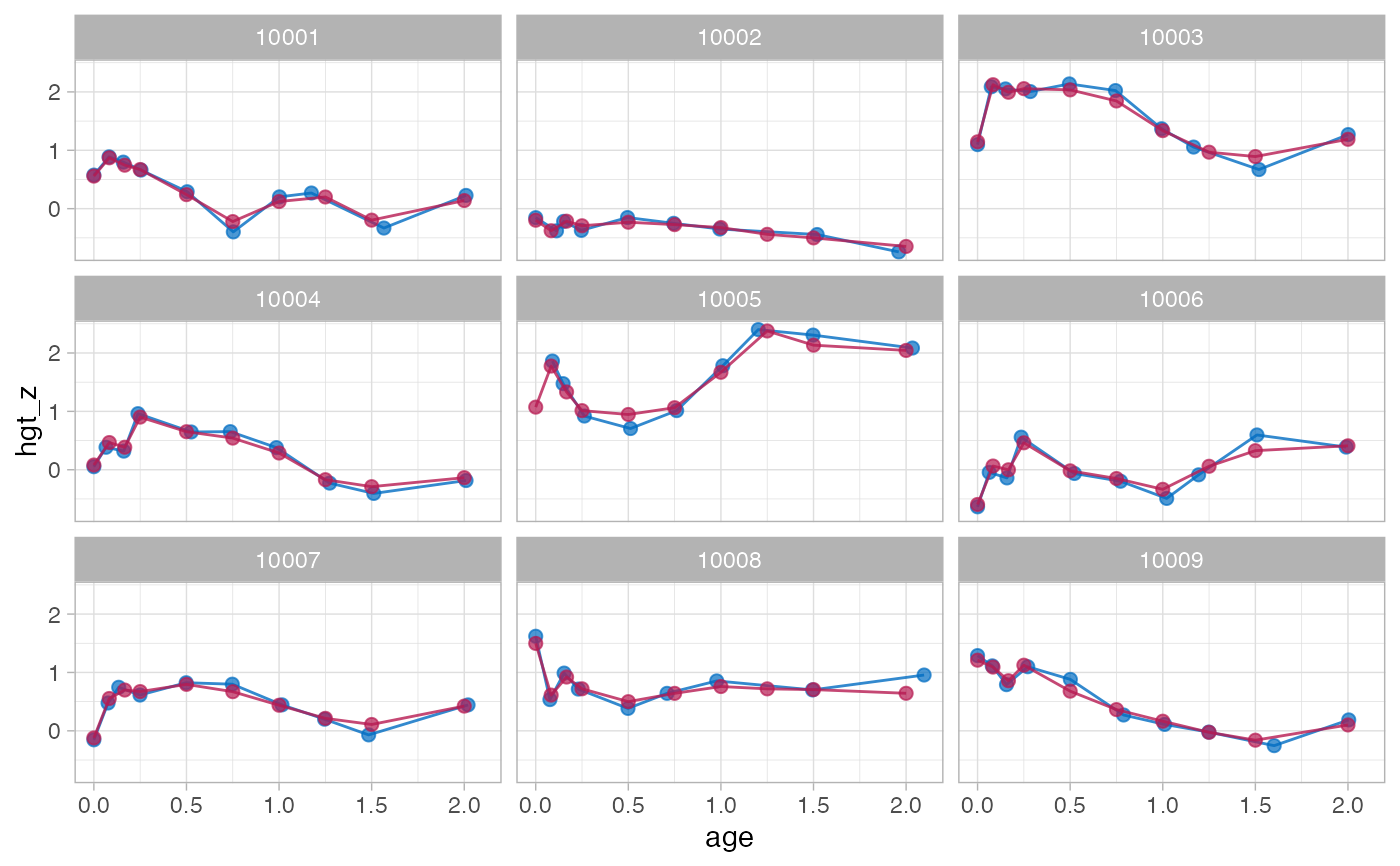
f3 <- brokenstick(hgt_z ~ age | id, data, knots, seed = 222)
plot(f3, data, n_plot = 9)


# method lmer takes about 40 seconds
f4 <- brokenstick(hgt_z ~ age | id, data, knots, method = "lmer")
#> Warning: number of observations (=1185) <= number of random effects (=1364) for term (0 + age_0 + age_0.0833 + age_0.1667 + age_0.25 + age_0.5 + age_0.75 + age_1 + age_1.25 + age_1.5 + age_2 + age_3 | id); the random-effects parameters and the residual variance (or scale parameter) are probably unidentifiable
#> boundary (singular) fit: see help('isSingular')
plot(f4, data, n_plot = 9)

# }