tanner: stage line diagrams and SDS for Tanner pubertal stages

This vignette covers material the README doesn’t have room for: a fuller plot_stadia() walkthrough across its main argument combinations, how raw testicular volume (tv) readings in ml are converted to a stage for plotting and SDS, and the statistical method behind calculate_sds() itself. For a quick installation and first-example walkthrough, see the README.

`plot_stadia()`: argument combinations

plot_stadia() draws one or more patients’ pubertal stage trajectories against the Dutch 1997 reference percentiles. Its main arguments are:

type: which of the three stage variables for a sex to plot (for boys: gen, phb, tv; for girls: bre, phg, men).
plotline: which of the same three reference percentile curves to draw in the background.
colors: the colors used for those three variables, matched positionally to type/plotline.
overlay: draw every person in persons on a single graph instead of one plot per person.
padid: append the patient id to the plot title.

A multi-timepoint boy, followed on genital stage, pubic hair, and testicular volume from age 9 to 15:

boy <- data.frame(
  id = 1,
  age = c(9.1, 10.2, 11.3, 12.1, 12.9, 13.8, 14.6, 15.2),
  sex = "M",
  gen = c(1, 1, 2, 3, 3, 4, 4, 5),
  phb = c(1, 1, 1, 2, 3, 4, 4, 5),
  tv = c(2, 3, 4, 8, 10, 12, 15, 20)
)

plot_stadia(
  data = boy,
  persons = 1,
  type = c(TRUE, TRUE, TRUE),
  plotline = c(FALSE, FALSE, FALSE),
  colors = c("#0060A0", "#00A000", "#A00000"),
  title = "Boy 1: genital, pubic hair & testicular volume",
  padid = FALSE
)

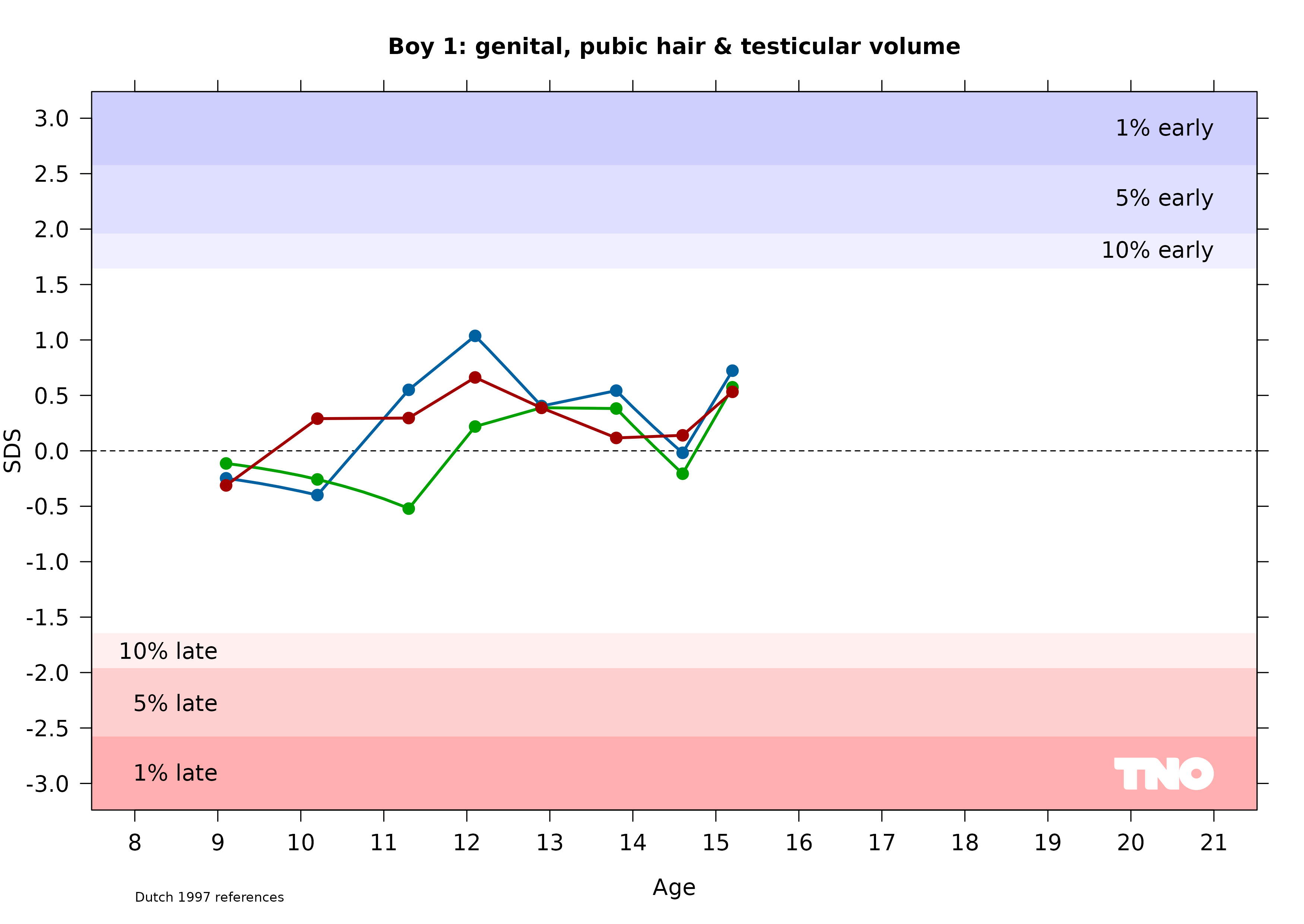
Here plotline is all FALSE, so only the patient’s own trajectories are drawn, without the background reference percentile curves — cleaner when several trajectories share one plot. The background curves (plotline) are independent of which trajectories are actually drawn (type): you can turn them back on to show, say, the tv trajectory alone against all three reference curves for context, with type = c(FALSE, FALSE, TRUE) and plotline = c(TRUE, TRUE, TRUE).

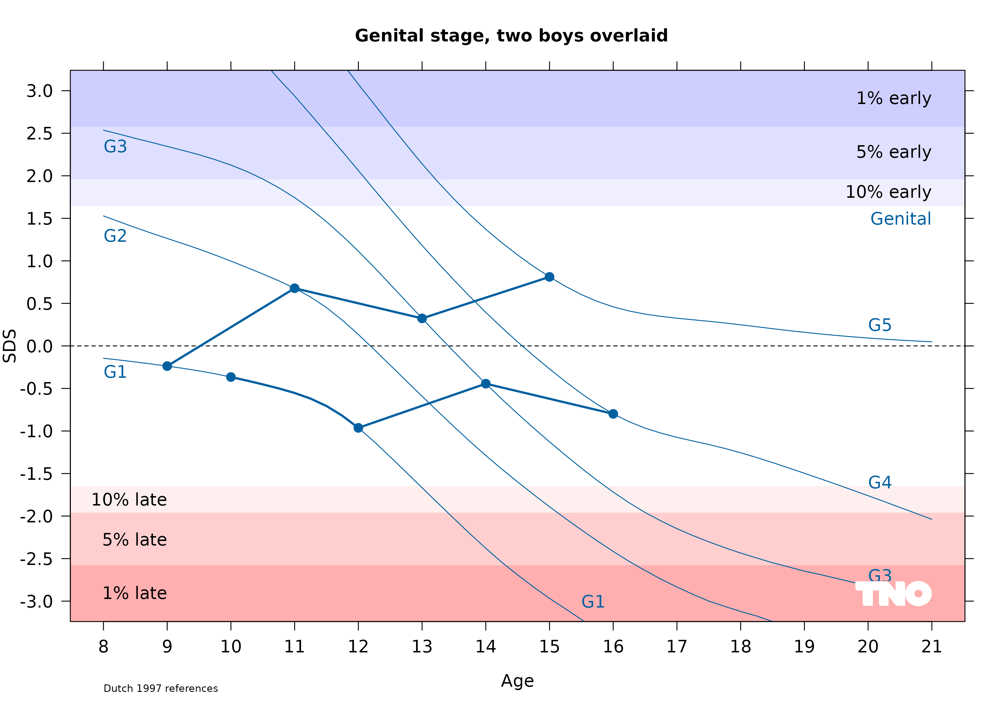
Comparing several patients with `overlay`

overlay = TRUE draws every person named in persons on one shared plot instead of a separate plot per person. Because a single plot only has one set of reference curves, overlay also takes ovsex to pick which sex’s percentiles to draw in the background — mixing sexes on one overlay plot only makes sense if you’re comparing trajectories against a single reference (or turning plotline off entirely):

boys <- data.frame(
  id = rep(c(1, 2), each = 4),
  age = c(9, 11, 13, 15, 10, 12, 14, 16),
  sex = "M",
  gen = c(1, 2, 3, 5, 1, 1, 3, 4),
  phb = c(1, 2, 3, 5, 1, 2, 3, 4),
  tv = NA
)

plot_stadia(
  data = boys,
  persons = c(1, 2),
  type = c(TRUE, FALSE, FALSE),
  plotline = c(TRUE, FALSE, FALSE),
  overlay = TRUE,
  ovsex = "M",
  title = "Genital stage, two boys overlaid",
  padid = FALSE
)

Testicular volume: a raw ml reading, not a bead index

tv (testicular volume) is recorded as a raw reading in ml, typically from a 12-point Prader orchidometer (1, 2, 3, 4, 5, 6, 8, 10, 12, 15, 20, 25 ml), but neither calculate_sds() nor plot_stadia() require the reading to land exactly on one of those 12 bead volumes — any plausible ml value works directly, with no recoding step.

The two functions handle a between-bead reading differently, because they answer different questions:

calculate_sds() needs a genuine percentile for the exact ml value, so it interpolates continuously. Internally it maps the raw ml reading onto a continuous bead-index scale (bead 1 = the T1/T2 curve¹, bead 2 = the next curve, and so on), rather than ml itself, because the beads are not evenly spaced in ml (1, 2, 3, 4, 5, 6, 8, 10, … — note the jump from 6 to 8). Interpolating in raw ml would make the SDS curve jump discontinuously right at each bead threshold; interpolating in bead index instead keeps it smooth across the whole ml range.
plot_stadia() (via the internal plot_stadia_data()) draws a trajectory as a single line following one reference curve, so a between-bead reading is snapped to whichever bead curve is nearest, rather than interpolated. A trajectory line can only trace one curve at a time.

# 11ml is strictly between the T10 and T12 Prader bead curves; age must
# be supplied per stage value (no recycling), so it's repeated here
calculate_sds(age = c(13, 13, 13), stage = c(10, 11, 12), type = "tv")

## [1] 0.3163986 0.4806011 0.6589934

The three SDS values increase smoothly and strictly monotonically with ml — 11ml’s SDS sits properly between 10ml’s and 12ml’s, rather than jumping or repeating a neighbor’s value.

The SDS methodology: mid-P values, not LMS

calculate_sds() implements the mid-P value method of van Buuren & Ooms (2009), which is worth understanding explicitly because it is not the LMS/BCCG/BCPE method most R users associate with growth-reference SDS (e.g. centile::y2z(), or the WHO/CDC growth charts). The two methods solve different problems:

LMS-style methods convert a continuous measurement (height, weight, BMI) to a Z-score against a continuously-varying reference distribution, typically fit via GAMLSS with L (skewness), M (median) and S (coefficient of variation) curves by age.
calculate_sds() converts a discrete/ordinal measurement — a Tanner stage (1 to 5), or a Prader bead-bracketed tv reading — to a Z-score. There is no continuous reference distribution to speak of: the reference data (nl1997) is a set of percentiles, one per age, at which a given fraction of the population has already reached a given stage.

Concretely, nl1997$gen holds, for each age, the fraction of boys who have not yet reached each genital stage:

head(tanner::nl1997$gen)

##    age     G2     G3 G4 G5
## 1 8.00 0.1152 0.0112  0  0
## 2 8.25 0.1317 0.0128  0  0
## 3 8.50 0.1494 0.0147  0  0
## 4 8.75 0.1681 0.0167  0  0
## 5 9.00 0.1875 0.0190  0  0
## 6 9.25 0.2079 0.0216  0  0

Column T3 at age 12, for example, is $P(\text{stage} < 3 \mid \text{age} = 12)$ — read directly off the reference table (interpolated between the nearest tabulated ages by calculate_sds()).

A patient observed at stage $c$ is treated as a coarsened observation of an unobserved, continuous latent variable — the “true” underlying developmental progress — that is uniformly distributed within the probability interval the observed stage covers:

$[P(Y < c \mid X),\ P(Y < c + 1 \mid X))$

The mid-P value is the mean of that latent variable:

$\pi_c = P(Y < c \mid X) + \frac{P(Y = c \mid X)}{2}$

which is equivalent to the average of the two surrounding “at least” percentiles:

$\pi_c = \frac{P(Y \geq c \mid X) + P(Y \geq c + 1 \mid X)}{2}$

and converting it to a Z-score is a single qnorm() call:

$Z = \Phi^{-1}(1 - \pi_c)$

This is why calculate_sds() averages the surrounding-stage percentiles rather than looking up a single stage’s percentile directly — the averaging is the mid-P value itself, derived from treating the stage as a coarsened continuous variable, not an ad hoc smoothing step bolted on afterward. The same formula applies unchanged to tv’s continuous ml scale (see above): the only difference is that the two percentiles being averaged come from continuous interpolation along the bead-index scale rather than a lookup at two adjacent integer stages.

Reference

van Buuren, S. and Ooms, J.C.L. (2009). Stage line diagram: An age-conditional reference diagram for tracking development. Statistics in Medicine, 28(11), 1569–1579. https://doi.org/10.1002/sim.3567

plot_stadia(): argument combinations

Comparing several patients with overlay

Testicular volume: a raw ml reading, not a bead index

The SDS methodology: mid-P values, not LMS

Reference

`plot_stadia()`: argument combinations

Comparing several patients with `overlay`