tanner

Tools to plot Tanner pubertal stage measurements against the Dutch 1997 references and express them as standard deviation scores (SDS).

This package implements the stage line diagram method described in:

van Buuren, S. and Ooms, J.C.L. (2009). Stage line diagram: An age-conditional reference diagram for tracking development. Statistics in Medicine, 28(11), 1569–1579. https://doi.org/10.1002/sim.3567

@article{vanbuuren-2009-1,
  title        = {Stage line diagram: An age-conditional reference diagram for tracking development},
  author       = {{van Buuren}, S. and Ooms, J.C.L.},
  year         = {2009},
  journal      = {Statistics in Medicine},
  volume       = {28},
  number       = {11},
  pages        = {1569--1579},
  doi          = {10.1002/sim.3567}
}

Package structure: library vs. webapp

tanner has two identities. plot_stadia() (and its helpers plot_stadia_general(), plot_stadia_lines(), plot_stadia_data()), interpolate_trajectory(), find_stage_segments(), calculate_sds() and tnologo() are the supported general-purpose library API: pure functions (or plotting functions taking explicit arguments) that anyone can library(tanner) and call interactively, covered by unit tests and this README’s walkthrough.

plotter(), plotterpro() and upload_tryCatch_pro() are rApache request handlers for the existing webapp deployment (see Production deployment (rApache)): they read GET/POST/FILES globals injected by rApache at request time and aren’t meant to be called interactively from R. They’re held to a lower bar — no unit tests, not part of this walkthrough — and kept exported only so the existing deployment keeps working.

This README covers three things:

1. Calculating SDS in plain R — no web app needed.
2. Running the local mock web app — try the browser frontends without setting up Apache/rApache.
3. Producing bulk diagrams with Puberty Pro — upload a whole dataset and get one PDF with everyone’s plot, plus a CSV/TXT of SDS values.

For the original production deployment (Apache + rApache), see Production deployment (rApache) at the end.

Installation

# from GitHub
install.packages("devtools")
devtools::install_github("growthcharts/tanner")

Or from a local clone:

install.packages("devtools")
devtools::install(".")

# or load without installing, from the repo root
devtools::load_all(".")

Example: plotting a stage line diagram

plot_stadia() draws a patient’s pubertal stage trajectory against the Dutch 1997 reference percentiles. Here’s a boy’s genital stage followed from age 8 to 16.5 (patient 7 from the original pubertal demo data.txt demo dataset used to produce genital.pdf/boy.pdf in this package’s source history):

library(tanner)

mydata <- data.frame(
  id = 1,
  age = c(
    8.10,
    8.37,
    8.58,
    8.87,
    9.12,
    9.34,
    9.58,
    9.86,
    10.11,
    10.36,
    10.59,
    10.86,
    11.15,
    11.34,
    11.59,
    11.88,
    12.13,
    12.36,
    12.61,
    13.13,
    13.63,
    14.16,
    14.66,
    16.13,
    16.53
  ),
  sex = "M",
  gen = c(
    1,
    1,
    1,
    1,
    1,
    1,
    1,
    1,
    1,
    1,
    1,
    1,
    1,
    1,
    1,
    1,
    1,
    2,
    2,
    3,
    3,
    3,
    3,
    4,
    4
  ),
  phb = NA,
  tv = NA,
  bre = NA,
  phg = NA,
  men = NA
)

plot_stadia(
  data = mydata,
  persons = 1,
  type = c(TRUE, FALSE, FALSE),
  plotline = c(TRUE, FALSE, FALSE),
  title = "Puberty Plot (patient 7, pubertal demo data.txt)",
  padid = FALSE
)

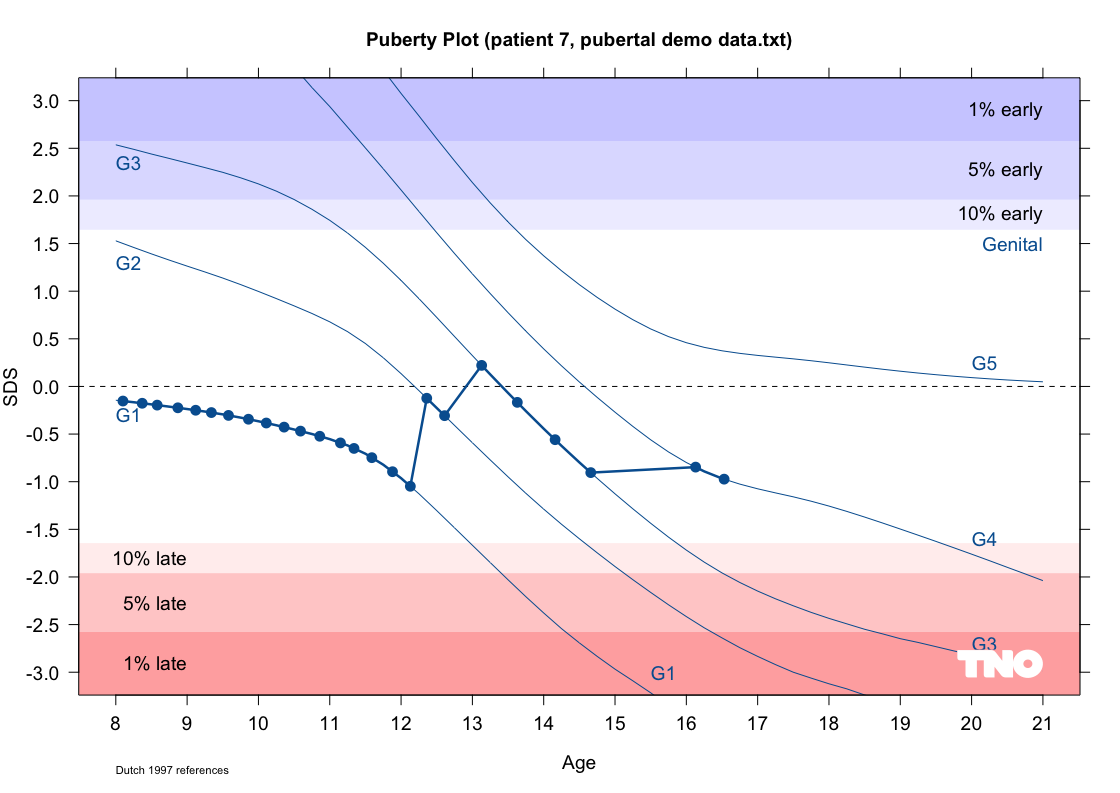
The shaded bands mark the 1%, 5% and 10% earliest/latest percentiles for the genital reference curve; the thick line is this patient’s own trajectory.

1. Calculating SDS in plain R

calculate_sds(age, stage, type) converts an age + observed pubertal stage into a standard deviation score, by interpolating the Dutch 1997 reference percentiles (nl1997). type is one of "gen", "phb", "tv", "bre", "phg" or "men".

library(tanner)

# a single measurement: a 12-year-old boy at genital stage 3
calculate_sds(age = 12, stage = 3, type = "gen")

[1] 1.11

Girls: bre / phg / men

bre and phg stages are coded 1–5, men is coded 1 (not yet) or 2 (menarche reached) — use them as-is:

girls <- read.csv("inst/webapps/pubertypro/demo.csv")
names(girls) <- tolower(names(girls))
girls$age <- as.numeric(gsub(",", ".", girls$age))
girls <- girls[girls$sex == "F", ]

girls$SDS_bre <- round(calculate_sds(girls$age, girls$bre, "bre"), 2)
girls$SDS_phg <- round(calculate_sds(girls$age, girls$phg, "phg"), 2)
girls$SDS_men <- round(calculate_sds(girls$age, girls$men, "men"), 2)

Boys: gen / phb / tv

gen and phb are coded 1–5 and can be used as-is. tv (testicular volume) is recorded in ml, typically read off a 12-point Prader orchidometer (1, 2, 3, 4, 5, 6, 8, 10, 12, 15, 20 or 25), but calculate_sds() and plot_stadia() accept any ml value directly — including readings between Prader beads (e.g. 11 or 16 ml) — by interpolating between the surrounding reference percentiles. No recoding needed:

boys <- read.csv("inst/webapps/pubertypro/demo.csv")
names(boys) <- tolower(names(boys))
boys$age <- as.numeric(gsub(",", ".", boys$age))
boys <- boys[boys$sex == "M", ]

boys$SDS_gen <- round(calculate_sds(boys$age, boys$gen, "gen"), 2)
boys$SDS_phb <- round(calculate_sds(boys$age, boys$phb, "phb"), 2)
boys$SDS_tv <- round(calculate_sds(boys$age, boys$tv, "tv"), 2)

Note: an age/stage combination can fall outside the plottable range (the SDS is effectively ±Inf for an extreme outlier, e.g. genital stage 1 at age 19). calculate_sds() still returns a value, but plot_stadia() will silently skip drawing a point for it, since it falls off the chart.

All six SDS at once on a mixed data.frame

calculate_sds() is vectorized, so a whole data.frame with both sexes can be processed in one go. Calling it on a stage column that doesn’t apply to a row (e.g. gen for a girl) just returns NA for that row, so there’s no need to split the data by sex first:

mydata <- read.csv("inst/webapps/pubertypro/demo.csv")
names(mydata) <- tolower(names(mydata))
mydata$age <- as.numeric(gsub(",", ".", mydata$age))

mydata$SDS_gen <- round(calculate_sds(mydata$age, mydata$gen, "gen"), 2)
mydata$SDS_phb <- round(calculate_sds(mydata$age, mydata$phb, "phb"), 2)
mydata$SDS_tv <- round(calculate_sds(mydata$age, mydata$tv, "tv"), 2)
mydata$SDS_bre <- round(calculate_sds(mydata$age, mydata$bre, "bre"), 2)
mydata$SDS_phg <- round(calculate_sds(mydata$age, mydata$phg, "phg"), 2)
mydata$SDS_men <- round(calculate_sds(mydata$age, mydata$men, "men"), 2)

This is the same calculation Puberty Pro runs for every uploaded dataset.

2. Running the local mock web app

inst/webapps/ ships two browser frontends (puberty for a single patient, pubertypro for batch upload). They were originally built to run behind Apache + rApache, which is now hard to set up on modern systems. tools/run_mock_webapp.R serves both frontends locally with httpuv, without needing Apache or rApache at all.

Install

install.packages("httpuv")
install.packages("devtools")   # only needed if you run from a source checkout

Start

From the repo root, in a terminal:

Rscript tools/run_mock_webapp.R

or, from an R/RStudio/Positron console, with the repo as the working directory:

source("tools/run_mock_webapp.R")

Either way it prints the URLs and opens the single-patient app in your default browser automatically:

Mock webapps running at:
  http://127.0.0.1:7654/puberty/
  http://127.0.0.1:7654/pubertypro/
Press Ctrl+C to stop.

Open http://127.0.0.1:7654/pubertypro/ yourself for the batch upload app — only the first URL is opened automatically.

Stop

• Terminal (Rscript): press Ctrl+C, or close the terminal.
• R console (source()): press Ctrl+C in the console (or the stop/interrupt button in RStudio/Positron) to break the server loop, or restart the R session.

If you try to start a second instance while one is still running, you’ll get Failed to create server / address already in use. Find and stop the process holding port 7654:

# macOS / Linux
lsof -nP -iTCP:7654 -sTCP:LISTEN
kill <PID>

# Windows (PowerShell)
Get-NetTCPConnection -LocalPort 7654 | Select-Object OwningProcess
Stop-Process -Id <PID>

3. Producing bulk diagrams with Puberty Pro

The pubertypro app processes an entire dataset (many patients) in one go: it draws one puberty plot per patient into a single multi-page PDF, computes SDS values for every measurement, and offers the result as a downloadable CSV/TXT alongside the PDF.

1. Start the mock server and open http://127.0.0.1:7654/pubertypro/.
2. Upload a data file. Sample files are linked on the page itself, and also available directly in the repo: inst/webapps/pubertypro/demo.csv, demo.sav, demo.txt. Required columns: id, age, sex ("M"/"F"), plus gen, phb, tv for boys and/or bre, phg, men for girls (NA-able per row).
3. Review the parsed per-patient summary table, then click GO!.
4. Download the generated files from the icon links:
   • PDF — one page per patient, with the puberty stadia plot (plot_stadia() under the hood).
   • CSV / TXT — the original data plus SDS_gen, SDS_phb, SDS_tv, SDS_bre, SDS_phg, SDS_men columns.

Doing the same thing from plain R, without the web app, looks like:

library(tanner)

mydata <- read.csv("inst/webapps/pubertypro/demo.csv")
names(mydata) <- tolower(names(mydata))
mydata$age <- as.numeric(gsub(",", ".", mydata$age))

pdf("all_patients.pdf", paper = "a4r", width = 11.67, height = 8.27)
plot_stadia(
  data = mydata,
  persons = unique(mydata$id),
  type = c(TRUE, TRUE, TRUE),
  plotline = c(FALSE, FALSE, FALSE),
  padid = TRUE
)
dev.off()

Production deployment (rApache)

The original deployment runs the webapps behind Apache with rApache:

# install R and the tanner package
R CMD INSTALL tanner_1.5.0.tar.gz

# install rapache, e.g. using the package
sudo apt-get install libapache2-mod-r-base

# copy the site file from the package and activate
sudo cp -Rf /usr/local/lib/R/site-library/tanner/sites-available/puberty /etc/apache2/sites-available
sudo a2ensite puberty

# restart apache
sudo service apache2 restart

# if anything isn't working, check the error log:
tail /var/log/apache2/error.log